
Since the introduction of gradient tree boosting methods, tree boosting methods have often been the highest performing models across many tabular benchmarks. Alongside this, they have often be the winning models in many Kaggle competitions. Today we’ll cover the most popular of these models: XGBoost.
XGBoost popularity stems from many reasons, with the most important being its scalability to all scenarios. It is one of the fastest tree based models to train because of the algorithms used with sparse data and it’s exploitation of parallel and distributed computing.
This article will follow a similar format to the XGBoost paper with the following sections being covered in this article:
- The Regularised Objective.
- The Split Finding Algorithms.
Constructing the Regularised Objective
Given a dataset with $n$ examples and $m$ features, $\mathcal{D} = \{(x_i, y_i)\} (|\mathcal{D}| = n, x_i \in \mathbb{R}^m, y_i \in \mathbb{R})$, a tree ensemble model uses K additive functions used to predict the output.
$$\hat{y}_i = \phi(x_i) = \sum_{k=1}^K f_k(x_i), \quad f_k \in \mathcal{F},$$where $\mathcal{F} = \{ f(x) = w_{q(x)} \}(q : \mathbb{R}^m \rightarrow T, w \in \mathbb{R}^T)$ is the space of regression trees, $T$ is the number of leafs in the tree, and each $f_k$ is a tree with its own tree structure $q$ and leaf weights $w$. Rather than taking the approach used by typical decision trees where each regression tree contains a continuous score on each leaf, we will use $w_i$ to represent score on the ith leaf. These scores are summed over the trees used in the prediction to give a final score:
$$\text{Prediction}(x) = \sum_{k=1}^K w_{k, q_k}(x)$$To learn these set of functions, we use the followed regularised objective:
$$\mathcal{L}(\phi) = \sum_i l(\hat{y}_i, y_i) + \sum_i \Omega (f_k) \quad \text{where } \ \Omega(f) = \gamma T + \frac{1}{2} \lambda \| w\|^2.$$Here, $l$ is a differentiable convex loss function (such as the mean squared error) and $\Omega$ is the complexity penaliser term to avoid overfitting. When the penalising term is removed, this objective function is the same as gradient boosting.
Gradient Tree Boosting
Tree ensemble methods cannot be optimised by traditional optimisation methods in the Euclidean space because they are discontinuos functions and are not differentiable. Consequently, this prohibits the use of gradient based optimisation methods which rely on these two properties. As a result, models need to be trained in an additive manner.
Given a prediction $\hat{y}_i^{(t)}$ of the ith instance (of $n$ samples) during the t-th iteration. We need to find $f_t$ that minimises this objective:
$$\mathcal{L}^{(t)} = \sum_{i=1}^n l(y_i, \hat{y}_i^{(t)} + f_t(x_i)) + \Omega(f_t).$$In essence, we greedily add the $f_t$ that improves our model the most.
Applying the Taylor’s Theorem Approximation, we can render a second-order approximation of the equation above:
$$\mathcal{L}^{(t)} \approx \sum_{i=1}^n [l(y_i, \hat{y}_i^{(t)}) + g_if_t(x_i)) + \frac{1}{2}h_if_t(x_i)^2] + \Omega(f_t),$$where
$$g_i = \frac{\delta l(y_i, \hat{y}_i^{(t-1)})}{\delta \hat{y}_i^{(t-1)} } \quad \text{and} \quad h_i = \frac{\delta l(y_i, \hat{y}_i^{(t-1)})}{\delta^2 \hat{y}_i^{(t-1)^2} }.$$Removing the constant terms gives:
$$\mathcal{L}^{(t)} = \sum_i^n [g_if_t(x_i)) + \frac{1}{2}h_if_t(x_i)^2] + \Omega(f_t).$$Let $I_j = \{i | q(x_i) = j \}$ be the instance set of the leaf $j$.
$$\mathcal{L}^{(t)} = \sum_{j=1}^T [(\sum_{i \in I_j}g_i)w_j) + \frac{1}{2}(\sum_{i \in I_j}h_i + \lambda) w_j^2] + \lambda T.$$Differentiating and equating to 0, tells us that the optimal weight $w_j^*$ of leaf $j$ is given by:
$$w_j^* = -\frac{\sum_{i \in I_j}g_i}{\sum_{i \in I_j}h_i + \lambda}.$$Substituting this above, gives the optimal value of:
$$\tilde{\mathcal{L}}^{(t)}(q) = -\frac{1}{2} \sum_{j=1}^T\frac{(\sum_{i \in I_j}g_i)^2}{\sum_{i \in I_j}h_i + \lambda} + \lambda T.$$This function can be thought of as a quality measure of the tree structure $q$ and can also be thought of as the impurity score.
The issue with this metric is that it becomes impossible to enumerate over all tree structures because any time a new branch is added, the number of potential configurations increases combinatorially. This approach is infeasible for any large dataset.
Alternatively, a greedy approach is taken where we start with a leaf and iteratively add branches to the tree. Let $I_L$ and $I_R$ denote the instance sets on the left and right nodes after the split. Letting $I = I_L \cup I_R$, then the loss reduction formula is given by:
$$\mathcal{L}_{\text{split}} = \frac{1}{2} \left[ \frac{(\sum_{i \in I_L}g_i)^2}{\sum_{i \in I_L}h_i + \lambda} + \frac{(\sum_{i \in I_R}g_i)^2}{\sum_{i \in I_R}h_i + \lambda} - \frac{(\sum_{i \in I}g_i)^2}{\sum_{i \in I}h_i + \lambda} \right] - \lambda.$$This formula is used for evaluating split candidates.
Shrinkage and Column Subsampling
In addition to the regularised objective, two further techniques were introduced by Tianqi Chen and Carlos Guestrin. The first method, is shrinkage introduce by Friedman where newly added weights are scaled by a factor $\mu$ after each step of tree boosting. This reduces the influence of each individual tree and leaves spaces for future trees to improve the model.
The second method is column subsampling (which is also used in random forest) and this method often outperforms the row sub-sampling method.
Split Finding Algorithms
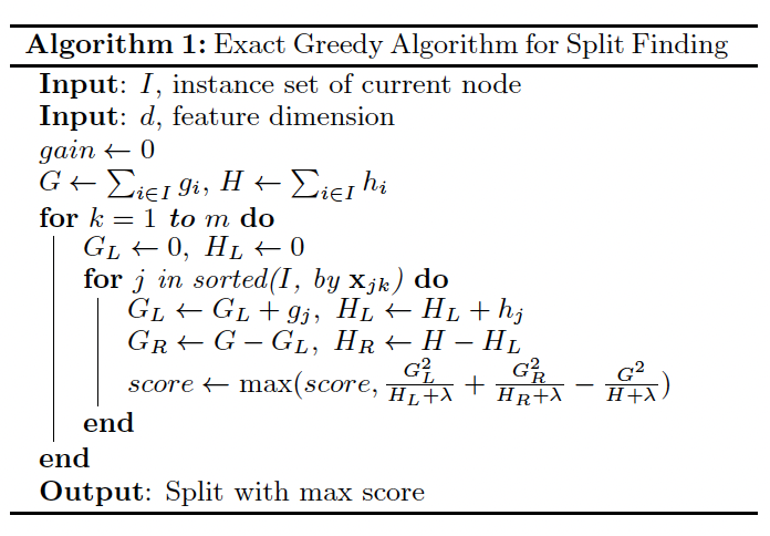
The basic split finding algorithm (which we will call the exact greedy method) which enumerates over all the possible splits on features is computationally demanding. This becomes even more of an issue when the dataset is large and does not fit into memory or if this model is trained in a distributive setting.
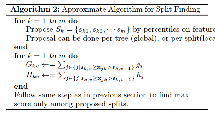
As a result, an alternative framework is proposed. This approximate algorithm proposes candidate split points based on percentiles of a feature distribution. The algorithm maps the continuous features into buckets split by the candidate split points, aggregates the statistics and finds the best solution among the proposals.
There are two variants of this proposal; the global variant which propose split points during the initial tree construction phase and then uses the same proposals for splits at each level. The local variant re-proposes after each split. The local proposal tends to outperform the global proposal, however, the global method can achieve a similar performance to the global proposal given enough candidate split points are given.
Most approximate methods for distributed tree learning also follow this framework but some construct approximations based on histograms of the gradient statistic and some use other variants of binning strategies instead of quantile. But, from these methods, Tianqi Chen and Carlos Guestrin chose to go for the quantile strategy.
Weighted Quantile Sketch
The most important step in each approximate algorithm is to find the best candidate split points. Usually, percentiles of a feature distribution are used to make candidates distribute evenly on the data. This methods did not incorporate any form of weighting and treated each data point as equally important. The limitations of this method, is that they assume uniform importance, which typically is not the case. This alternative method incorporates the hessian information into its splitting.
Formally, for a multi-set $\mathcal{D}_k = \{ (x_{1k}, h_1), ..., (x_{nk}, h_n) \}$, which represents the kth feature values and second order gradient statistics for each training class. The rank function $r_k: \mathbb{R} \rightarrow [0, \infty)$ as:
$$r_k(z) = \frac{1}{\sum_{(x, h) \in D_k} h} \sum_{(x, h) \in D_k, x < z} h,$$which represents the proportion of instances whose feature value $k$ is smaller than $z$. The goal is to find candidate split points $\{ s_{k1}, s_{k2}, ..., s_{kn}\}$ such that:
$$|r_k(s_{k,j}) - r_k(s_{k,j+1})| < \epsilon, \quad s_{k1} = \min_i x_{ik}, \quad s_{kl} = \max_i x_{ik}.$$Where $\epsilon$ is an approximation factor. This means that there is roughly $1/\epsilon$ candidate points and here, each data point is weighted by the hessian $h_i$.
We use the hessian as the weighting because it captures the importance uncertainty of each data point within the optimisation setting:
- Curvature information. The Hessian captures the curvature of the loss function. A higher. curvature (large $h_i$) implies that the gradient at this point is changing more rapidly and the model should focus on these points because they may impact the model’s performance.
- Weight Squared Loss. The rewritten loss takes the form of: $\sum_{i=1}^n \frac{1}{2} h_i \left(f_t(x_i) - \frac{g_i}{h_i} \right)^2 + \Omega(f_t) + \text{constant}$, which is a weighted square loss with labels $g_i/h_i$.
- The gradient is insufficient. The gradients $g_i$ indiciate the direction of optimisation but does not account for the magnitude or stability of the loss function. If only the gradient points were used as weights the model would be unable to distinguish between instances with similar gradients but different curvatures (uncertainty). This could lead to suboptimal splits that do not accurately capture the structure of the data.
The algorithm for the approximate splitting algorithm is below.
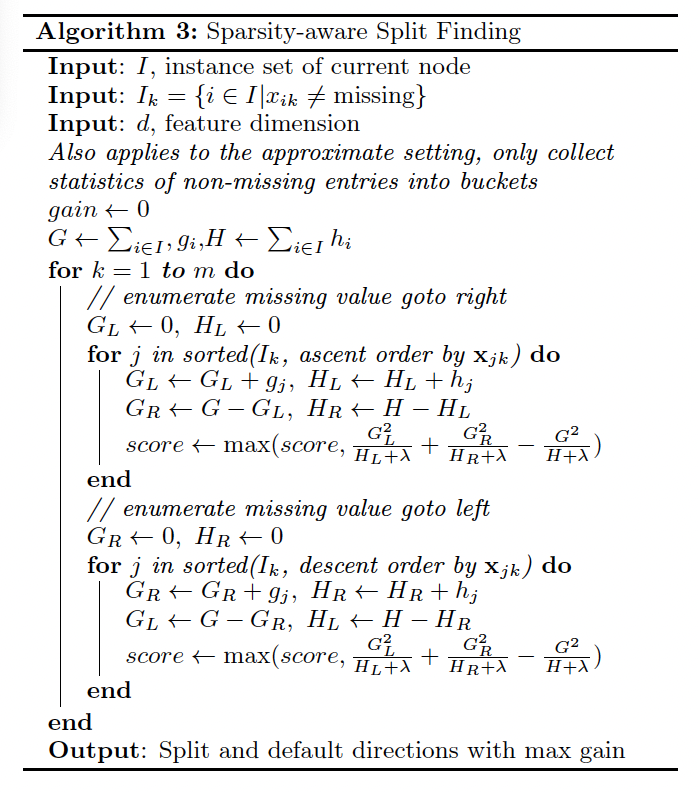
Sparsity-aware Split Finding
In many of the real world problems, the input $x$ is sparse as a result of the presence of missing values, frequent zero entries, or artefacts a result of feature engineering and one hot encoding. To make an algorithm aware of this sparsity, Tianqi Chen and Carlos Guestrin proposed to add a default direction in each tree. When a sample is missing, the instance is assigned to that direction with the optimal direction learnt from the data.
Conclusion
In todays article we covered the maths behind the leading tree boosting algorithm, XGBoost. In later articles we will cover the system design behind XGBoost and its end-to-end evaluations.