Over the past 15 years we have seen a surge of use of Graph Neural Networks (GNNs) being used to model social networks, recommendations systems, transportation networks, and many more systems. With the ever growing use of GNNs, this has naturally led to the questions about the use of GNNs within the medical sector. More specifically, the question of using GNNs to predict the properties of molecules was brought up. Back in the early 2010s, this idea was in its infancy with few successful applications.
Similarly, in the 2010s, we observed significant advancements in large-scale quantum chemistry calculations and molecular dynamics simulations (see the appendix for more details). Coupled with the increased speed of experimentation, these advancements have led to the generation of vast amounts of data. To effectively harness this data, more powerful models became necessary. One promising approach was the use of Neural Network (NN) architectures, which have demonstrated great success in handling large datasets and modelling complex interactions.
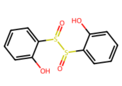
However, molecules present a unique challenge. They tend to be irregular in structure and do not fit well into traditional grid or sequential formats, making them non-Euclidean in nature. To effectively model molecules, a graph-based representation is needed, where atoms are treated as nodes and chemical bonds as edges. This naturally leads to the consideration of GNNs.

Figure 1. An example molecule from the PyTorch MoleculeNet dataset.
The second main drive behind using GNNs to model molecules comes from the GNN’s inductive bias of permutation invariance. In short, this means that if a different permutation of the same molecule entered the model the same prediction would be given. Most other classes of Neural Networks lacked this property making the GNNs preferable.
Even with these preferences towards GNNs, there was one limitation present. Many of the GNNs before 2017 did not incorporate edge information in their message passing system. Consequently, a new GNN-like architecture had to constructed, this led to Gilmer et al. constructing the class of NNs called the Message Passing Neural Networks (MPNNs).
The MPNN Framework
Given a undirected graph $G$, we will denote with node features of node $v$ as $x_v$ and edge features as $e_{vw}$ where $w \in \mathcal{N}(v)$. The MPNN framework can be broken down into two phases: the message passing phase and the readout phase.
The message passing phase is run for T steps and is defined by the differentiable message function $M_t$ and differentiable vertex update function $U_t$. This message passing phase updates the hidden states of node $v \ (h_{v}^{t})$ using the message $m_{v}^{t+1}$:
$$m_{v}^{t+1} = \sum_{w \in \mathcal{N}(v)} M_{t}(h_{v}^{t}, h_{w}^{t}, e_{vw}),$$$$h_{v}^{t+1} = U_{t}(h_{v}^{t}, m_{v}^{t+1}).$$The readout phase is implemented in the final layer of the MPNN. This computes a feature vector for the whole graph using a differentiable readout function $R$ according to:
$$\hat{y} = R(\{h_{v}^{T} | v \in G\} ).$$These outputs $\hat{y}$ of the readout function are then fed into a neural network to solve the classification or regression problem.
GG-NN
Before jumping into Gilmer et al.’s model, it is worth mentioning many other GNNs could be considered suitable MPNNs. Specifically, the GNN called Gated Graph Neural Networks (GG-NN) by Li et al. was used as the baseline for Gilmer et al. choice of model.
In the GG-NN architecture, the message passing system and the update function is defined as:
$$M_{t}(h_{v}^{t}, h_{w}^{t}, e_{vw}) = A_{e_{vw}}h_{w}^{t},$$$$U_{t} = GRU(h_{v} ^{t}, m_{v} ^{t+1})$$where $A_{e_{vw}}$ is a learned matrix and GRU stands for the Gated Recurrent Unit by Cho et al. This work implemented weight tying which constricts the update function to remain the same for every time step t.
Finally the readout function takes the form:
$$\begin{equation}R = \sum_{v\in V} \sigma \left( i(h_{v}^{T}, h_{v}^{0}) \right) \odot \left( j(h_{v}^{T})\right),\end{equation}$$where $i$ and $j$ and neural networks, $\odot$ denotes the element wise multiplication, and $\sigma$ denotes an activation function (often being the sigmoid activation function).
Gilmer et al.’s MPNN
The first modification made to the GG-NN model was in the message-passing function. Here, Gilmer et al. defined the message function as $M_{t}(h_{v}, h_{w}, e_{vw}) = A(e_{vw}) h_{w}^{t}$, where $A(e_{vw})$ is a neural network that maps edge vectors $e_{vw}$ to a $d \times d$ matrix referred to as the edge network. This design introduced the feature that the message produced depends solely on the embedding of node $w$, $h_{w}^{t}$, and not on the current embedding of node $v$, $h_{v}$. This design choice was made to simplify the computational process. Alternatively, a more computationally expensive method would involve passing the message from node $w$ to node $v$ along their edge using $m_{wv} = f(h_{w}^{t}, h_{v}^{t}, e_{vw})$, where $f$ is a neural network.
For the readout function, two options were explored. The first was identical to the one implemented in the GG-NN model (equation 1) and the second option was inspired by the set2set model by Vinyals et al. In the second approach, the model performs a linear projection on each tuple $(h_{v}^{t}, x_{v})$, then stores the results of these projected tuples $T = \{(h_{v}^{T}, x_{v})\}$. After $M$ steps of computation, the graph generates a graph-level embedding, $q_{t}^{\star}$ from these tuples. This final operation is invariant to the order of the tuples and the resulting embedding is then fed into a neural network.
During Gilmer et al’s training, the best performing model used the set2set readout function.
The final innovations centred around the introduction of virtual graph elements, aimed at improving the message-passing capabilities of the model by facilitating the transfer of information over longer distances. The first idea introduced a virtual edge type for each pair of nodes that were not directly connected. The second method involved adding a master node that was connected to every node in the graph via a unique edge type. This master node had a separate dimensionality and separate weights for its update function.
The limitation of this method revolves around its complexity. A single step in the MPNN for a dense graph requires $\mathcal{O}(n^{2} d^{2})$ operations where $n$ in the number of nodes and $d$ is the dimension of the node embeddings. This is a consequence of the message passing step where each node embedding message suffers from complexity $\mathcal{O}({d}^{2})$ and this operation is performed $n^{2}$ resulting in the complexity of $\mathcal{O}(n^{2} d^{2})$. To solve this issue, the node embeddings can be broken down into k different embeddings of size d/k denoted by $h_{v}^{t+1, k}$. The propagation step is running on each k copies generating node embeddings $\tilde{h}_{k} ^{t, k}$ and then these embeddings are then mixed together via a neural network:
$$(h_{v}^{t, 1}, h_{v}^{t, 2}, ... , h_{v}^{t, k}) = g(\tilde{h}_{v}^{t, 1}, \tilde{h}_{v}^{t, 2}), ... , \tilde{h}_{v}^{t, k}),$$where $g$ denotes the neural network and $(x, y, ...)$ denotes the concatenation. Using this method, each k embeddings part achieves a complexity of $\mathcal{O} (n^{2} (d/k)^{2})$ and multiplying this result by the k different embedding parts gives a complexity of $\mathcal{O} (n^{2} d^{2} / k)$.

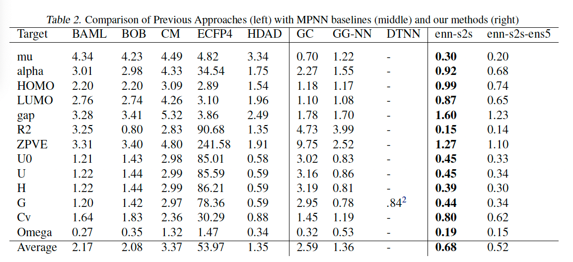
Figure 2. The performance of Gilmer el al’s MPNN model with a set2set readout function. enn-s2s denotes the best model and enn-s2s-ens5 denotes the ensemble model with an ensemble of 5 different predictions. The right side corresponds to the benchmarks for GNNs in molecule prediction tasks such as polarity and energy level predictions. Source found here: Gilmer, J., Schoenholz, S., Riley, P., Vinyals, O. and Dahl, G. (n.d.). Neural Message Passing for Quantum Chemistry. [online] Available at: https://arxiv.org/pdf/1704.01212v2.
Limitations of MPNNs
Looking at figure 2 we can see that the Gilmer et al’s MPNN exceeded the performance of the previous state of the art model on the tested benchmarks, however, even with this strong performance, there were some notable limitations.
- The MPNN struggled to generalise effectively to graphs that are larger than those encountered during training. This is particularly problematic in domains like chemistry, where molecules of varying sizes need to be analysed.
- Any approaches that utilize spatial information in MPNNs tend to create fully connected graphs, where each node is connected to every other node. As a result, computing the number of message can be computationally expensive.
Conclusion
This article introduced the idea of the MPNN, a form of GNN with applications in molecule prediction problems.
Appendix
Quantum Chemistry: Quantum chemistry use the quantum mechanical principles to calculate the properties and behaviours of molecules at the atomic level. These used to be computationally expensive, but due to recent advancements in computational power, these form of calculations are now possible to be performed at a large scale.
Molecular dynamics simulations: Molecular dynamics (MD) simulations model the physical movements of atoms and molecules over time. These simulations are used to predict how a molecule will evolve within different conditions. Similar to the quantum chemistry, advancements in computational power has made these calculations possible.
References
Gilmer, J., Schoenholz, S., Riley, P., Vinyals, O. and Dahl, G. (n.d.). Neural Message Passing for Quantum Chemistry. [online] Available at: https://arxiv.org/pdf/1704.01212v2.
Li, Y., Zemel, R., Brockschmidt, M. and Tarlow, D. (n.d.). Published as a conference paper at ICLR 2016 GATED GRAPH SEQUENCE NEURAL NETWORKS. [online] Available at: https://arxiv.org/pdf/1511.05493 [Accessed 14 Aug. 2024].
Chung, J., Gulcehre, C. and Cho, K. (2014). Empirical Evaluation of Gated Recurrent Neural Networks on Sequence Modeling. [online] Available at: https://arxiv.org/pdf/1412.3555.
Vinyals, O., Bengio, S., Kudlur, M. and Brain, G. (n.d.). ORDER MATTERS: SEQUENCE TO SEQUENCE FOR SETS. [online] Available at: https://arxiv.org/pdf/1511.06391 [Accessed 4 Sep. 2024].
