 Image by Elijah Grimm
In this article we will cover the ARMA and ARIMA based statistical models, cover the maths behind these models, and look at the statistical test required prior and the post the model fitting.
I’d recommend reading the previous article here before reading the remainder of this article. In that article we cover the basics of what is a time series and how we could model it.
Definitions:
Recall from our previous article that given a sequence of data points $\{ X_{t}, t \in \mathbb{Z} \}$, the sequence is strongly stationary or strictly stationary if
$$\left( X_{t_{1}}, \dots, X_{t_{k}}\right) \overset{d}{=} \left( X_{t_{1} + h}, \dots, X_{t_{k} + h}\right),$$for all the time points $t_{1}, \dots, t_{k}$ and integer $h$ [1]. A sequence is weakly stationary or second order stationary if
$$\begin{aligned} \mathbb{E}(X_{t}) &= \mu \\ \text{and} \quad \text{Cov}(X_{t}, X_{t+k}) &= \mathbb{E}[(X_{k} - \mu)(X_{t+k} - \mu)] = \gamma_{k}, \end{aligned}$$where $\mu$ is constant and $\gamma_{k}$ is independent of $t$ and the sequence $\{ \gamma_{k}, k \in \mathbb{Z} \}$ is called the autocovariance function. At the lag 0, $\gamma_{0} = \mathbb{E}[(X_{k} - \mu)^{2}] = \text{Var}(X_{k})$.
In general, a process is $X_t$ is stationary if the autocovaraince function $\gamma_k$ does not depend on $t$.
These definitions will be useful later in the article.
Indeterministic Processes
There are many other processes in time series other than stationarity, one of these processes are indeterministic processes. A process is purely-indeterministic if the regression on $X_{t-q}, X_{t-q-1}, \cdots$ has explanatory power tending to 0 as $q \rightarrow \infty$, i.e. the ability for the regressors to explain the variable $X_t$ diminishes to 0. Alternatively, this can be expressed as the residual variance of the series tends to $X_t$.
The key feature of these processes is that no matter how much past data is acquired, there will always be a sense of randomness in the data.
In any forecasting in the real world, there will alway be a random element introducing uncertainty into the model. ARMA based models account for this randomness by incorporating error terms which we will now cover below.
ARMA
Given a stationary process $\{X_t\}$, an autoregressive moving average process ARMA(p, q) is defined as
$$X_t - \sum_{r-1}^p \phi_r X_{t-r} = \sum_{s=0}^{q} \theta_s \epsilon_{t-s},$$where $\{ \epsilon_t \}$ is white noise. The parameter p corresponds to the autoregressive component where the current value depends on its previous p values and the parameter q corresponds to the moving average component which is influenced by the last q noisy terms.
Finding the parameters p and q of the ARMA(p, q) model can be found by plotting the partial autocorrelation functions (PACF) and autocorrelation functions (ACF) respectively. Alternatively, both of these parameters can be determined using the extended autocorrelation function (EACF) which excels in situations where the parameters indicated by the PACF and ACF plots fail to provide clear indication on which parameters should be used.
PACF
Given a time series $X_t$, the partial autocorrelation of lag k, denoted as $\phi_{k,k}$ is the autocorrelation between $X_t$ and $X_{t+k}$ with $X_{t+k-1}$ removed. In other words, it is the autocorrelation between $X_t$ and $X_{t+k}$ which is not accounted by lags 1 to k-1. This stems from the idea that the terms $X_t$ and $X_{t-k}$ are indirectly dependent on $X_{t-1}, X_{t-2}, \cdots, X_{t-k+1}$ and if they are not removed, the partial autocorrelated will not capture the true correlation between $X_t$ and $X_{t+k}$.
$$\phi_{1,1} = corr(X_{t+1}, X_t), \quad \text{for } k= 1, ...$$$$\phi_{k,k} = corr(X_{t+k} - \hat{X}_{t+k}, X_t) - \hat{X}_t, \quad \text{for } k \geq 2,$$where $\hat{X}_{t+k}$ and $\hat{X}_{t}$ are linear combinations of $\{ X_{t+1}, X_{t+2}, \cdots, X_{t+k-1}$ that minimise the mean square error of $X_{t+k}$ and $X_t$ respectively. Specifically,
$$\hat{X}_{t+k} = \beta_1 X_{t+k-1} + \cdots + \beta_{k-1} X_{t+1} \quad \text{and} \quad \hat{X}_t = \beta_1 X_{t+1} + \cdots + \beta_{k-1} X_{t+k-1}.$$These parameters can be calculated with the Durbin-Levinson Algorithm which is an algorithm that recursively calculates the solution to an equation using the Toeplitz matrix. More details about this algorithm can be found here.
EACF
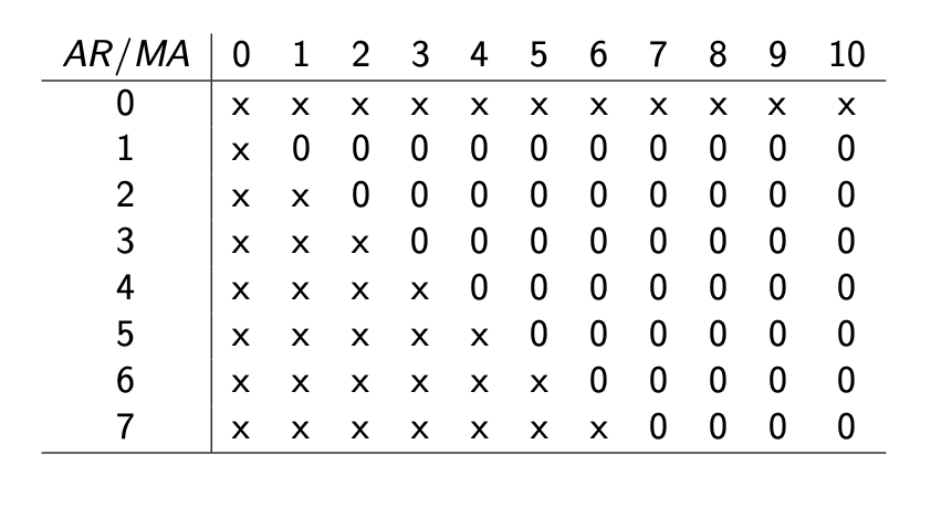
The EACF [2] is a two dimensional table that compares the lags of different AR and MA components. The rows correspond to the different values for the AR component p and the columns correspond to the different MA components q.
Each entry in the table is given a 0 if the residuals at ARMA(p, q) are approximately white noise and are given an X if there is an indication of a poor fit.

To assign 0 to a parameter combination, we can approximate the autocorrelation of the residuals to a $N(0, 1/(n-p-q))$ distribution where we subtract the parameter p and q to reduce the bias in our estimation of the variance. These parameters are subtracted because there are p and q parameters which are unknown. If the sample autocorrelation surpasses $1.96/\sqrt{n-p-q}$ then there is sufficient evidence to suggest the residuals are not white noise and the model has failed to capture the process’s information.
Estimating the parameters of an ARMA model
Once the correct hyperparameters p and q have been chosen, the next step is to determine the parameters of the model. The most common method for this is Maximum Likelihood Estimation (MLE), which finds the parameters that maximize the likelihood of observing the actual time series data. This process begins with an initial guess for the parameters, followed by computing the likelihood of the observed data given those parameters. Optimization algorithms such as Gradient Descent, Newton-Raphson, or BFGS are then used to iteratively adjust the parameters to improve the likelihood. These algorithms rely on the gradient and sometimes the second derivative (Hessian) of the likelihood function to guide parameter updates until convergence is achieved. Statistical packages such as “statsmodels” in Python employ these methods, and once the model is fitted, diagnostics like residual autocorrelation and parameter uncertainty are checked to validate the model.
It is worth mentioning other estimation methods could be used instead of MLE such as the Generalised Least Squares (GLS) or Method of Moments (MoM). However, in practice, these methods are often disregarded in favour for the MLE.
These diagnostic methods include checking the residual autocorrelations and assessing the normality of the residuals. If the model is well-fitted, the residuals should be uncorrelated, which can be tested using the Ljung-Box test or by inspecting the ACF of the residuals. To evaluate the normality of the residuals, you can use a Shapiro-Wilk test, a Q-Q plot, or a Jarque-Bera test (see the appendix).
Evaluating your ARMA model
Now that the model has been fitted, the next step is to evaluate the residuals of the model. If the model has been fit well, the residuals should behave like white noise (i.e. the mean of the residuals should be zero and should not have a pattern). There are a few different tests to test the residuals
First is the Ljung-Box test[4] which test the group of autocorrelations of a time series are different from 0. Rather than testing the randomness at each lag, it test the “overall” randomness based on a number of lags. The test goes as follows.
Null Hypothesis (H0): The data is independently distributed.
Alternative (H1): The data is not independently distributed and exhibit serial correlation.
The test statistic is written as
$$Q = n(n+2) \sum_{k=1}^h \frac{\hat{\rho}_k^2}{n-k},$$where n is the sample size, $\hat{\rho}_k$ is the autocorrelation at a lag k, and h is the number of lags being tested. Under H0, the statistic should asymptotically follows a chi squared distribution with degrees of freedom h $\mathcal{X}^2_h$. Consequently, to reject the null:
$$Q > \mathcal{X}^2_{1-\alpha, h}.$$It is important that the degrees of freedom $h$ must be adjusted based on the parameters $p$ and $q$ to $h -p - q$.
Alternatively to the Ljung-Box test, a Jarque-Bera test could be used [5]. A Jarque-Bera test is a goodness-of-fit test which tests whether the residuals follow a normal distribution. In general, if residuals are not normally distributed, the current model may not be accounting for all the patterns in the data. For more details about this test, please refer to the appendix.
ARIMA
In many situations, the modelled process will not be stationary. Consequently, the process will need to be made stationary using a differencing process. A first order differencing operation for distribution $\{X_t\}$ is expressed as
$$Y_t = \nabla X_t = (X_t - X_{t-1}).$$Similarly, a second order differencing is expressed as
$$Y_t = \nabla^2 X_t = (X_t - X_{t-1}) - (X_{t-1} - X_{t-2}) = X_t - 2X_{t-1} + X_{t-2}.$$A process $Y_t$ is said to be an autoregressive integrated moving average process, ARIMA(p,d,q) if $Y_t = \nabla^d X_t$ is an ARMA(p,q) process.
These ARIMA models have some well known cases [1] such as
- An ARIMA(0,1,0) model $X_t = X_{t-1} + \epsilon_t$ is a random walk.
- An ARIMA(0,1,0) model with a constant $X_t =\mu + X_{t-1} + \epsilon_t$ is a random walk with a drift.
- ARIMA(0,0,0) is a white noise model.
- ARIMA(0,1,2) is the Damped Holt’s model.
- ARIMA(0,1,1) is a basic exponential smoothing model.
In general, ARMA models assumes the data is stationary while for ARIMA models the time series may not be stationary. ARIMA will use this differencing procedure to make the data stationary and from here follow the ARMA based modelling procedure.
Conclusion
Today we covered a few key definition within time series. Additionally, we covered ARMA based models and the process required to ensure the correct parameters have been chosen for our model.
Appendix
Gaussian Processes: A Gaussian process (GP) is a process where $X_{t_1}, \cdots, X_{t_n}$ has a joint normal distribution for all $t_1, \cdots, t_n$. No two distinct Gaussian processes will have the same autocovariance function.
GPs are non-parametric model used to forecast time series data by modelling the time series as a collection of random variables that follow a Gaussian distribution. Not only will these model create predictions but will also provide uncertainty estimates. These uncertainty estimates can then be applied to create confidence intervals for each prediction.
As mention in the last paragraph, these models are non-parametric because they take no explicit assumptions on the structure of the timer series. Instead, they use a kernel function to model the relationship between data points.
This kernel function can take many forms, one common kernel function is the squared exponential kernel which is used to model smooth continuous trends in time series data.
GPs excel in situations where the data’s relationship is complex or unknown and when uncertainty measures are required.
**Jarque-Bera test **. A Jarque-Bera test is a goodness-of-fit test which tests whether the residuals have skewness and kurtosis matching a normal distribution. The test statistic (called JB) is non-zero and when it is far from 0, the residuals do not follow a normal distribution.
$$JB = \frac{n}{6}(S^2 + \frac{1}{4}(K-3)^2 ),$$where n is the number of observations, S the sample skewness, and K the sample kurtosis.
$$S=\frac{\hat{\mu}_3}{\hat{\sigma}^3} = \frac{\frac{1}{n}\sum_{i=1}^n (x_i - \bar{x})^3}{(\frac{1}{n}\sum_{i=1}^n (x_i - \bar{x})^2)^{3/2}},$$$$S=\frac{\hat{\mu}_4}{\hat{\sigma}^4} = \frac{\frac{1}{n}\sum_{i=1}^n (x_i - \bar{x})^4}{(\frac{1}{n}\sum_{i=1}^n (x_i - \bar{x})^2)^{2}},$$where $\hat{\mu}_3$ and $\hat{\mu}_4$ correspond to the estimates of the 3rd and 4th central moments. If the residuals follow a normal distribution, than the JB statistic will asymptotically achieve a chi squared distribution. In general, samples from a normal distribution should have expected skewness of 0 and an expected kurtosis of 0 (same as a kurtosis of 3).
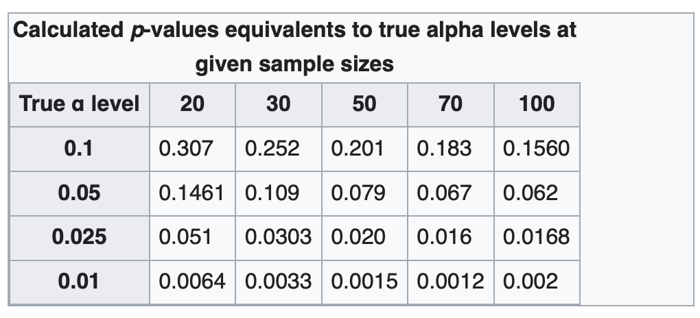
Some example rejection regions for this test are below.

Figure 2. Rejection Regions in JB test. Source found at: https://en.wikipedia.org/wiki/Jarque–Bera_test
References
- TIME SERIES Contents. (n.d.). Available at: https://www.statslab.cam.ac.uk/~rrw1/timeseries/t.pdf.
- Chapter 6: Model Specification for Time Series. (n.d.). Available at: https://people.stat.sc.edu/hitchcock/stat520ch6slides.pdf.
- Wikipedia Contributors (2019). Autoregressive integrated moving average. [online] Wikipedia. Available at: https://en.wikipedia.org/wiki/Autoregressive_integrated_moving_average.
- Wikipedia Contributors (2023). Ljung and Annelund. [online] Wikipedia. Available at: https://en.wikipedia.org/wiki/Ljung.
- Wikipedia. (2020). Jarque. [online] Available at: https://en.wikipedia.org/wiki/Jarque.